Dynamic Causal Modeling (DCM) takes a probabilistic Bayesian framework to infer effective or causal connectivity, essentially to model how a stimulus would influence the connectivity between regions.
In the previous blogpost we looked at some of the fundamental aspects of Bayes’ theorem. In this blog we look at one application of a Bayesian approach to EEG/MEG data, known as dynamic causal modeling (DCM) [1], which is used to infer effective connectivity. Effective connectivity aims to estimate the influence of one neural region over the other (i.e. causal influence), as opposed to functional connectivity that aims to seek statistical associations (or correlations) [2].
Starting with the Inverse Problem
DCM was originally proposed for fMRI data analysis, but in this blog we will keep the focus on EEG/MEG data, as the underlying principles largely remain the same (except for the way in which the models are specified). The main idea in DCM analysis is about model inversion. We are already familiar with the concept of EEG inverse problems, where the aim is to estimate the neural activity x, given EEG/MEG data y. We have previously seen that the EEG/MEG data can be modeled as
![]()
Where L is the lead-field matrix that captures the assumptions of how currents from the dipoles are transformed into electric potential recorded at EEG sensors, x is the unknown neural activity and n is the measurement noise. This is also known as the forward model.
DCM analysis casts this problem in a probabilistic framework, and instead of just estimating the neural activity, it asks the question – suppose the system (i.e. the brain) is perturbed by a known external stimulus, can we infer how the connectivity between the brain regions is influenced ?
Based on a nonlinear model for how each brain region interacts
DCM first assumes a model for how activity within each brain region evolves and interacts with each other and also accounts for the presence of a stimulus. This is modelled using what are known as neural mass models, which are essentially a set of nonlinear differential equations that describe the interaction between the sub-population of the cortical region, that may include various cells. Mathematically, this can be written as

Let us not worry about the exact form of the function f() (which is given by neural mass models), but just understand here that DCM assumes that the neural states evolve in time according to this nonlinear model, where u is the input stimulus, 𝛳 are the model parameters that model the connectivity between the brain regions (and also intrinsic connections within! ) and x, the hidden neuronal states. Essentially DCM assumes an experimental stimulus as a perturbation of neuronal dynamics and such stimulus can change the connectivity (and neuronal activity), which can be inferred using Bayesian approaches.
The neuronal states are then propagated to the EEG sensors, again according to the forward model that we have seen before.
![]()
An example of using DCM to model mismatch negativity
Now the task in DCM is to infer x and 𝛳, given y. One of the fundamental differences between DCM and other connectivity estimation approaches is that, in DCM you have to specify a set of competing models (i.e. hypothesis) about how your data is generated. For examples, consider an example for mismatch negativity experiment, where you expect to see a negative peak in EEG when deviant sounds are encountered in a stream of repeated sounds and this occurs at about 100-200 ms [3]. Another aspect about DCM is that it assumes the locations of the brain regions to be known a priori and in this case five sources five sources over left and right primary auditory cortices (A1), left and right superior temporal gyrus (STG), and right inferior frontal gyrus (IFG) are thought to be involved, based on literature related to source localization in mismatch negativity. What is shown below is a set of three competing models F-model, B-model and FB-model. As you can see, each model assumes that the connectivity due to an input stimulus that is relayed through auditory cortices modulates the connectivity between the brain regions in a different manner. Now which model do we place our trust on ?
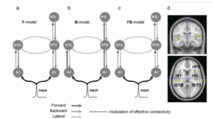
Figure 1 : Competing models to explain mismatch negativity [3]
Bayesian inference at play
This is precisely the question DCM tries to answer using a combination of Bayesian approaches that involves Bayesian inference and model selection. Thus given a model m, DCM aims at model inversion. In Bayesian parlance, the aim is to estimate the posterior distribution p(𝛳,x|y,u,m), given the likelihood(i.e., the forward model) p(y|𝛳,x,u,m) and some prior probability distribution over the parameters and neuronal state, i.e., one’s beliefs about this parameter, before any data is seen.
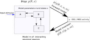
Figure 2 : Given a model m about how three brain regions (A,B,C) modelled using neural mass models interact, where 𝛳 is the unknown connectivity between (or even within) the brain regions and x are the hidden neuronal states, DCM aims to infer these quantities using Bayes’ theorem — i.e., based on likelihood model and a prior distribution over 𝛳 and x.
The figure below summarizes the main ingredients in DCM. In the next blogposts, we will look at neural mass models and how Bayesian inference and model selection are actually performed within DCM.

Figure 3: Main steps involved in DCM analysis. Figure re-interpreted from SPM course slides.
Some Caveats
Note that there are a lot of assumptions at play at every step from the dipole behavior of the sources to the neural mass model f() to a priori knowledge of connections between brain regions. Also, it might be difficult to specify competing models for a large number of brain regions. Its always good to examine assumptions and not accept them at face value.
References
[1] Friston, K. J., Harrison, L., & Penny, W. (2003). Dynamic causal modelling. Neuroimage, 19(4), 1273-1302.
[2] Friston, K. J. (2011). Functional and effective connectivity: a review. Brain connectivity, 1(1), 13-36.
[3] Kiebel, S. J., Garrido, M. I., Moran, R. J., & Friston, K. J. (2008). Dynamic causal modelling for EEG and MEG. Cognitive neurodynamics, 2(2), 121-136.
An important aspect of DCM for EEG is that since the data are the distribution of the electrical field at the sensors, one can compare models with different (numbers of) regions, which is not the case for DCM for fMRI (or DCM with reconstructed sources in EEG).
Additionally, the influence of a deep region (i.e. thalamus) has been sometimes modeled as an hidden one, see Boly M, Moran R, Murphy M, Boveroux P, Bruno MA, Noirhomme Q, Ledoux D, Bonhomme V, Brichant JF, Tononi G, Laureys S, Friston K. Connectivity changes underlying spectral EEG changes during propofol-induced loss of consciousness. J Neurosci. 2012 May 16;32(20):7082-90. doi: 10.1523/JNEUROSCI.3769-11.2012. PMID: 22593076; PMCID: PMC3366913.