A Bayesian framework, one that works with conditional probabilities, has numerous applications in Neuroimaging in general and in EEG specifically. But first, a primer on Bayes theorem and how it works.
The Bayesian approach has several applications in the field of EEG data analysis. For instance, several models of neuronal interactions can give rise to the same EEG outcome. Which model or hypothesis is the most probable ? Also, can we reduce the uncertainty about our models by integrating previously acquired domain knowledge ? These things (and much more) can be answered within the context of a Bayesian framework. Another application would be to formulate the EEG inverse problem in a probabilistic manner and use Bayesian approach to estimate the distributions of source currents from EEG data.
Frequentist versus Conditional Probabilities
The most common notion of probability that we are familiar with is that it represents the frequency of outcomes when an experiment is performed many times. For example, if we flip a coin 1000 times, we will expect to get heads about 500 times. This notion, based on the long run frequencies of events, is known as the frequentist interpretation of probability.
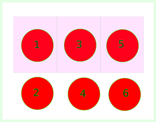
The Bayesian interpretation of probability rests on the notion of using probability to quantify uncertainty about something. Before understanding what Baye’s theorem means, let us quickly familiarize ourselves with the ideas of joint, conditional and marginal probabilities. Imagine that there are six balls numbered 1 to 6. Let A denote the event of picking up ball number 5 and B denote the event of picking up an odd numbered ball (see Figure 1). 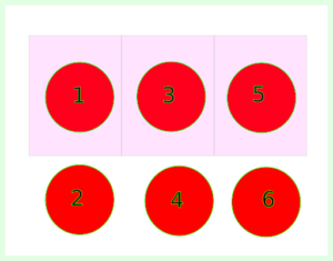
Now if one can ask a question – What is the probability of picking up ball number 5, given that you have picked up an odd number? Mathematically, what we aim to compute is P (A | B), i.e. probability of A given B has occurred. This seems pretty straightforward to compute. Since we know that B has occurred, this means either 1, 3 or 5 has been picked. Now the probability of the picked ball being 5 is simply 1/3. This can also be given using a formula,
P(A|B) = P(A,B) / P(B)
Where P(A,B) is the probability that both A AND B have occurred, which in our case would simply be 1/6 and the probability that only B has occurred, i.e., P(B) is 1/2 (because out of six possible outcomes, only three outcomes can be an odd number), thus P(A|B) = 1/6 / 1/2 = 1/3
The term P(A|B) is also referred to as conditional probability and P(B) is known as marginal probability. Once can analogously define,
P(B|A) = P(A,B) / P(A)
Bayes theorem
Using the above two equations, we arrive at the Baye’s theorem, which tells us that
P(B|A) = P(A|B) * P(B) / P(A)
Ok! Now what does this tell us and how is this useful? Now it looks like we are simply multiplying some probabilities and dividing by some probability?
Let us unpack this formula and what it can do with a concrete example. Assume that there is a test that is capable of detecting disease D. Now it is known that the test is 90% accurate. That is, 900 out of 1000 people who have this disease will test positive. Also, it is known that the test will give a positive reading even in the absence of the disease in 8% of the cases. We also know that it is a rare disease and its occurence in the population is 1%, i.e.P(D) = 0.01. Thus P(D*) = 1-0.01 = 0.99, which denotes the percentage of the population that does not have the disease.
Now you have taken the test and the result has come out as positive. You are very likely to believe the result. After all, the test is 90% accurate. However, is this a correct deduction ? Well, as per the Baye’s theorem, you have to refine your answer a bit!
Let us visualize the whole scenario using a diagram. Assume that you have the disease and thus you belong to the red area in Figure 2. Now you take the test and the result could either be +ve or -ve. In this scenario, the probability that it will be positive is 0.90 as the test has an accuracy of 90%, thus we can define the conditional probability P(+ve|D) = 0.90. Consequently P(-ve|D), i.e. you will test negative given you have the disease has to be 0.10, since total probability should sum to 1.
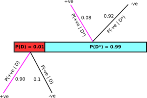
Similarly, if you do not have the disease (and hence belong to the cyan section), again two scenarios are possible – you will test positive and the probability of this happening, denoted by P(+ve|D*) is 0.08 (as we know that the test gives false positives 8 out of 100 times). Consequently, the probability of test coming out negative, given that you do not have the disease is P(-ve|D*) = 0.92. Now that we are armed with all this information and probabilities, we are interested in knowing – What is the probability that I have the disease, given that the screening i +ve ? That is, what is P(D|+ve) ? Baye’s theorem to the rescue!
According to Baye’s theorem (see the equation above)
P(D|+ve) = P(+ve|D) P(D) / P(+ve)
We have access to the two terms in the numerator, i.e., P(+ve|D) = 0.90 and P(D) = 0.01 . What about the term P(+ve) –the probability of screening positive overall ? We can calculate this by adding along the magenta colored branches above, which lead to the situation of screening positive no matter whether you have the disease or not.
Thus, P(+ve) = P(+ve|D) P(D) + P(D*)P(+ve|D*) = 0.90*0.01 + 0.99*0.08 = 0.0882. Plugging these values to the equation above, we arrive at P(D|+ve) ≈ 0.10 . In other words, if you test positive, you only have about a 10% chance of actually having the disease, despite the test accuracy being 90%!
In Bayesian terminology, P(D|+ve) is known as posterior probability and P(D) is known as the prior belief. Now you can reduce your uncertainty enormously, by getting tested again as your prior probability of having disease, P(D), is now 10 percent rather than 1 percent. If your second screening also comes out to be positive, applying Bayes’ theorem will now yield P(D|+ve) = 0.53, i.e. 53%! Thus, iterating Bayes’ theorem using updated prior beliefs can yield extremely precise information. In contrast, frequentist interpretation doesn’t attempt to calculate quantities like P(disease|+ve).
In the coming blogposts, we will see some of the applications of Baye’s theorem in neuroimaging data analysis.