How do you compare and select the best Bayesian model in Dynamic Causal Modeling or DCM of EEG data?
In the previous two blogs we learnt about the basic components of dynamic causal modelling (DCM) with electroencephalography (EEG) and looked at two key components – neural mass models and Bayesian inference in some detail. In this two-part blog post we will look at Bayesian model selection in detail.
The Bayes factor
As we have discussed before, in DCM one has to specify competing candidate models or hypotheses. Thus, we need a way to eventually compare these models and select the model that best explains our data. Just to recap, these models are described using a population of neural mass models with unknown connectivity parameters. Bayesian model selection is used in DCM to evaluate the relative probabilities of these models given the EEG/MEG data we want to analyze the connectivity for, and any prior information available on the model. For a given model mi and MEG/EEG data y, p(mi|y ) represents the conditional probability of model mi given the data y. If there are N such models, the task is then to choose the best model.

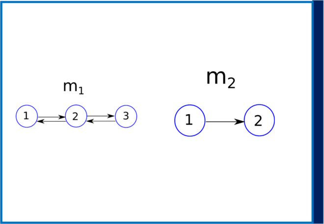
Figure 1 : Two candidate models m1 with three interacting brain regions and m2 with two interacting brain regions.
As an example let us consider that there is only one model m1 and the prior p(𝛳|m1). In this scenario, the posterior distribution of unknown parameters (i.e. the connectivity between brain regions as specified by the model) is given as,

Now suppose instead of one model, you have two competing models m1 and m2 (see Figure1). Now the question arises, which is the best model among these two after we have observed the data y? Bayesian model selection can be used in this scenario. This requires us to compute the posterior probabilities p(m1|y) and p(m2|y), which simply indicates that given the data (and any prior), which model do we trust more, m1 or m2? From Bayes’ theorem we have,
![]()
Comparing the two models, we have

The plausibility of the two models m1 and m2 can thus be evaluated using the ratio of the marginal likelihoods p(y|mi) also known as model evidence, which is also known as Bayes factor,

A value B12 > 1 can be interpreted as favoring model 1 over model 2 given the observed data y. Similarly, B12 < 1 would mean that we would want to favor model 2 over model 1, given the data y. To gain more intuition on this, it is also useful to observe at this point that we can write the ratio of the posterior probabilities p(m1|y) and p(m2|y) as,

From the above equation we can see that the ratio of probabilities of two models m1 and m2 have changed after we have seen the data (i.e., the posterior probabilities), is given as the Bayes factor times the ratio of the prior models’ probabilities. Thus, regardless of our prior beliefs on the two models (we may favour one model over the other before we see the data), the Bayes factor gives the factor by which we have to update our beliefs in the two models after seeing the data! In other words, posterior odds = Bayes factor X prior odds [1]. The interpretation of Bayes factor values in comparing two models is given in the following table [1-2]
| B12 | p(m1|y) | Evidence in favor of m1 |
| 1-3 | 0.5-0.75 | Weak |
| 3-20 | 0.75-0.95 | Positive |
| 20-150 | 0.95-0.99 | Strong |
| >=150 | >=0.99 | Very strong |
Thus, given two models m1 and m2, a Bayes factor of 150 would correspond to a belief of 99% in favor of model m1, whereas a Bayes factor of 3 would correspond to a belief of 75%.
In the next blog post, we will look at interpreting and gaining some intuition on the model evidence, on which the Bayes factor depends. We will also look at some applications of DCM to EEG/MEG and certain issues with using Bayes factor.
[1] Kass, Robert E., and Adrian E. Raftery. “Bayes factors.” Journal of the american statistical association 90.430 (1995): 773-795.
[2] https://www.fil.ion.ucl.ac.uk/spm/course/slides14-may/11_DCM_Advanced_1.pdf