This post discusses the core components of neural mass models and Bayesian inference in DCM applied to EEG.
In the previous blogpost we looked at the main components of dynamic causal modelling (DCM) for EEG data. Here we will look at the core components of DCM – neural mass models and Bayesian inference in some detail. To recap, the main steps involved in DCM for EEG are

Figure 1: Main steps involved in DCM analysis. Figure re-interpreted from SPM course slides.
Neural mass models
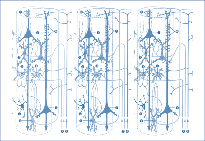
The model specification in DCM involves specifying multiple hypotheses about how different cortical regions interact with each other. Each cortical region is modelled using what are known as neural mass models – a mathematical model describing the dynamics of a cortical region. Specifically, it is a set of ordinary differential equations that describe the interaction between the sub-population of the cortical region, that may include for example inhibitory interneurons, excitatory interneurons and pyramidal neurons.
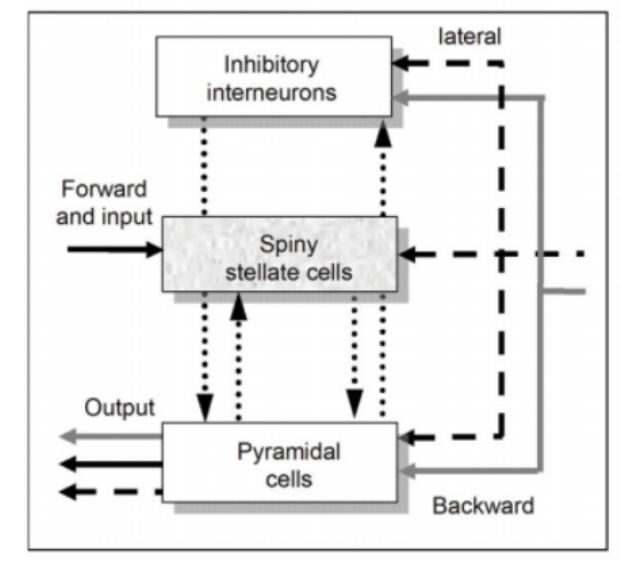
Figure 2: Each neural mass modeled can be described as a theoretical construct of interaction between various sub-populations of neuron sand can include both backward and lateral connections [1]
Neural mass models were originally proposed by Jansen and Ritt [2] to model the dynamics of a cortical column. Today many extended versions of this model (with more number of coupled differential equations!) are commonly used to model the generation of EEG/MEG activity. We won’t get into the details of the neural mass models and their validity (but for a thorough read refer [3-4] and see also The Crisis of Computational Neuroscience and Glia as Key Players in Network Activity)
At this point, for the purpose of understanding the methodology, each neuronal source in this model is represented using a set of differential equations that have several parameters with some biological significance. These parameters include synaptic gain, average number of synaptic contacts between the sub-populations etc [3-4].
Imagine we have two neuronal sources that are interacting with each other. Mathematically, this can be modelled using two neural mass models, with interaction between them modelled as additional parameters. In general, we can model N number of neural sources interacting with each other using a population of neural mass models, as shown in the figure below, where for simplicity we assume that each population has only pyramidal neurons and inhibitory interneurons, with Kij representing the connectivity between population i and j, and ad representing the connection delay [4].
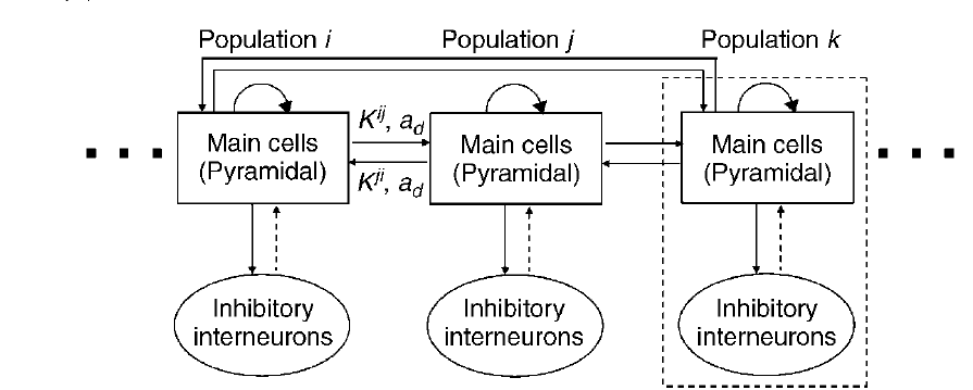
Figure 3 : Schematic representation of a population of neural mass models [4]
Bayesian inference
Now that we have specified our candidate models, the next step is to perform model inversion, i.e., given the EEG/MEG data and other known parameters find the unknown parameter that best fits the data. This is where a Bayesian approach known as variational Bayes is used. Since Bayesian approaches treat unknown parameters as random variables, what is inferred is a probability distribution over the parameters, rather than a single value. One can also specify a prior probability distribution for the parameters that would express one’s beliefs or assumptions about this parameter, before any data is seen.
Recall the Bayes’ theorem, which is given as
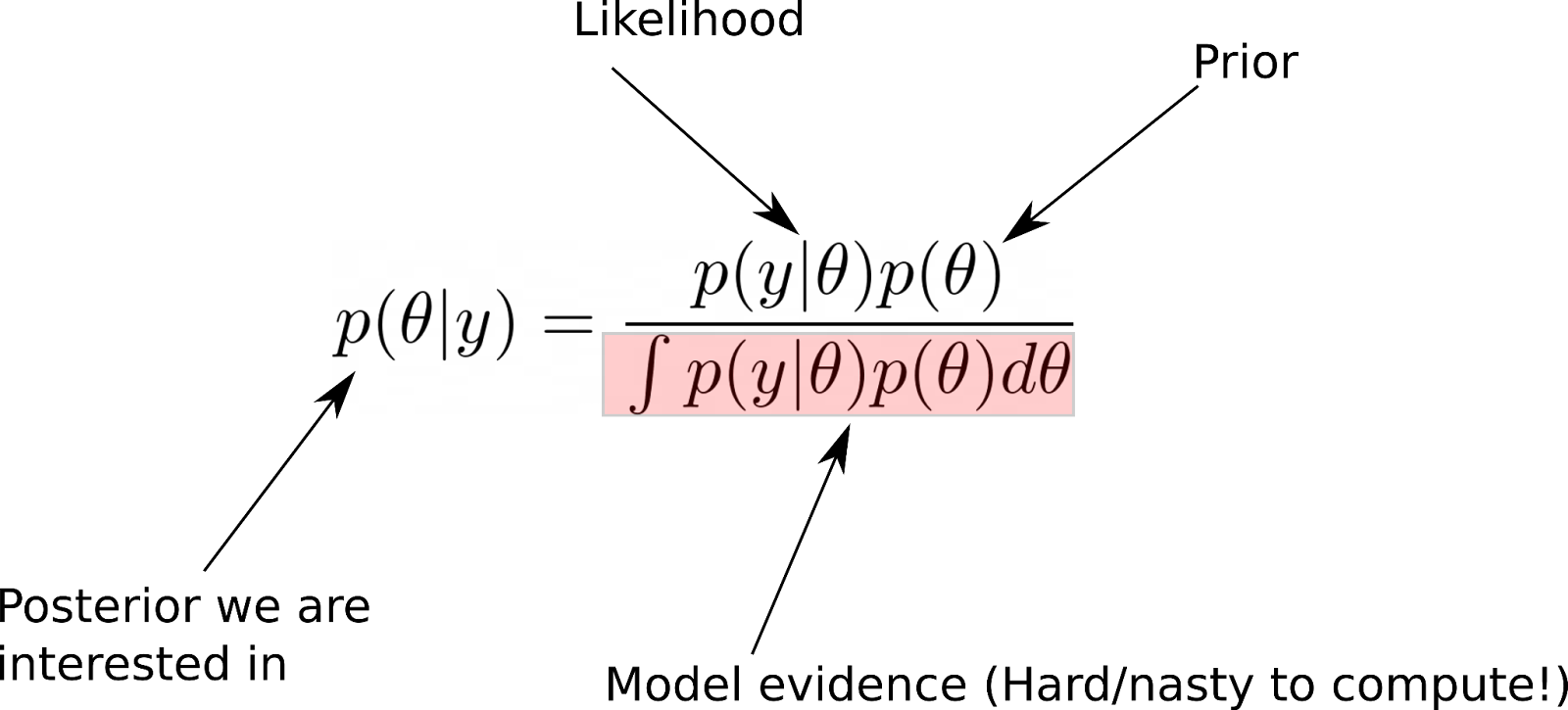
Figure 3 : The Bayes’ theorem
Where p(y|𝛳) is the likelihood (i.e., the forward model in EEG that expresses how unknown parameters 𝛳 of the neural sources are mapped to the EEG data y) and p(𝛳) is the prior distribution over the parameters. The denominator, also known as the model evidence, nothing but the marginal probability p(y) ( See A Primer of Bayes Theorem for Neuroimaging).
Let us suppose that there are N candidate models m1 to mN that we wish to test. The first task then is to estimate the posterior distribution of 𝛳 for each m, i.e., p(𝛳| y, m) (In DCM along with parameters that states x are also estimated, but for simplicity we will refer to p(𝛳,x | y, m) as p(𝛳| y, m)) . In many cases, this distribution cannot be obtained in closed form as it is very hard to compute the denominator in the above equation, which can include high-dimensional integrals, which cannot be solved analytically. In DCM, an approximation approach known as variational Bayes algorithm [5] is used, where the aim is slightly less ambitious – rather than find the true posterior distribution, try to find a distribution from a family of distributions that is as close as possible to this true posterior distribution.
Okay – so how do we measure this closeness ? Luckily, there is a simple way to do this — using what is known as the Kullback-Leibler divergence! You can kind of think of this as a distance measure, but for probability distributions. But unlike a distance measure, this is not a symmetric measure. That is, for any two probability distributions p(𝛳) and q(𝛳), the KL divergence between p(𝛳) and q(𝛳) is not equal to the KL divergence between q(𝛳) and p(𝛳). If you are interested in the more technical aspects of the algorithm, there are many references available (for example see [5]). For now, we will stick to the simplistic explanation that the VB algorithm first initializes q0(𝛳) from a family of distributions Q and then iteratively tries to minimize the KL divergence. In the figure below, after certain iterations we find a distribution q*(𝛳), that has the smallest KL divergence to the true posterior p(𝛳| y, m). But wait, p(𝛳| y, m) depends on the model evidence p(y), which is hard to compute , so how can we measure the KL divergence between q(𝛳) and p(𝛳| y, m) ?
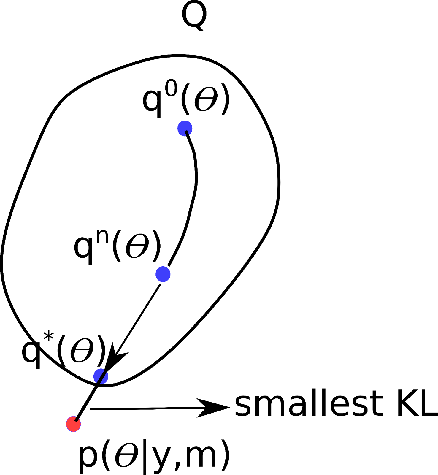
Figure 5 : Schematic of the iterative optimization in variational Bayes’ algorithm
Here is where things get a little complicated mathematically. Actually, what happens under the hood of the variational Bayesian algorithm is that KL divergence is minimized by actually maximizing another quantity. After a bit of mathematical manipulation,we can express model evidence as a sum of two quantities
Model evidence = L + KL divergence (q(𝛳), p(𝛳| y, m))
Since KL divergence is always greater than or equal to 0 (it is zero when q(𝛳) = p(𝛳| y, m)), model evidence > L. This term L is known as evidence lower bound (ELBO) (also known as negative variational free energy), as it is indeed the lower bound of the model evidence. When we try to maximize the ELBO , we are in turn minimizing the KL divergence, with the best case of KL divergence being equal to zero!
So those were the two important steps in DCM in a nutshell. In the next blogpost, we will look at how Bayesian model selection (i.e., choosing the best models given a set of candidate models) is performed in DCM, along with some applications to EEG data.
References
[1] Kiebel, S.J., Garrido, M.I., Moran, R., Chen, C.-C. and Friston, K.J. (2009), Dynamic causal modeling for EEG and MEG. Hum. Brain Mapp., 30: 1866-1876. https://doi.org/10.1002/hbm.20775
[2] Jansen, B.H. & Rit, V.G. (1995) Electroencephalogram and visual evoked potential generation in a mathematical model of coupled cortical columns.Biol. Cybern., 73, 357±366.
[3] Wendling, F., et al. “Epileptic fast activity can be explained by a model of impaired GABAergic dendritic inhibition.” European Journal of Neuroscience 15.9 (2002): 1499-1508.
[4] Wendling, F., and P. Chauvel. “Transition to ictal activity in temporal lobe epilepsy: insights from macroscopic models.” Computational neuroscience in epilepsy. Academic Press, 2008. 356-XIV.
[5] Blei, D. M., Kucukelbir, A., & McAuliffe, J. D. (2017). Variational inference: A review for statisticians. Journal of the American Statistical Association, 112(518), 859–877.