Beamformers, a technique adapted from radar applications, are a type of spatial filtering approach to solving the inverse problem in EEG and MEG. Here are the basics of how it works.
In the previous blog posts, we explored the EEG/MEG inverse problem and the different approaches to solve them. To recap, the aim of solving an EEG/MEG inverse problem is to estimate the location, orientation and strength of neural sources (which are usually modelled as dipoles), given the EEG/MEG measurements.
Approaches to the inverse problem
There are three broad categories of approaches to solve the EEG/MEG inverse problem, 1) dipole fitting, 2) distributed source imaging and 3) spatial filtering. The three ingredients for solving an inverse problem are 1) Source model – which assumes sources (for example modelled as dipoles) to be either on the cortical surface or even the entire brain volume, 2) Lead-field matrix or forward model – a model that explains how the source space with dipoles of unit strength, produces EEG/MEG measurements, given the different head tissues. 3) EEG/MEG measurement data.
Beamformers: a spatial filtering approach
In this blogpost, we will focus on a spatial filtering approach, known as beamformers, a technique introduced originally for radar applications. Beamformers actually describe an array of antenna elements, arranged in a specific way so as to add the incoming (or outgoing) signals in a preferred direction but cancel each other out in other directions, thus giving an antenna array a spatial directivity [1]. The figure below illustrates the basic idea underlying spatial filtering, where a spatial beamformer weights the output of the sensors x1 to xN at time t to give an output y(t). The weights w1 to wN are chosen such that signals from a desired direction are enhanced and from other directions are suppressed. Stacking everything in a vector form, we can represent the output of the spatial beamformer as:
![]()
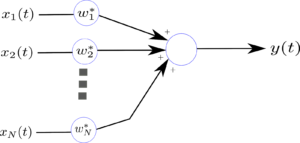
Figure 1 : Illustration of a spatial beamformer
How are beamformers useful in EEG/MEG source estimation ?
The property of beamformer to selectively enhance signals coming from a particular direction is exploited for the estimation of the neuronal sources from EEG/MEG measurements.
Let us assume that we have the volume conductor model of the head obtained using some numerical methods such as FEM or BEM. The figure below illustrates the basic idea. Here m1 to m151 are MEG sensors. The weights w1 to w151 is assigned to each sensor and the neuronal source at a location of interest is then constructed as a weighted sum of the MEG sensors. The aim here is then to choose the weights in such a way that on the signal from the location of interest contributed to the beamformer output and the signal from other locations (which are considered as interference or noise) are suppressed [2]. Note that a different set of weights is computed for each dipole location.
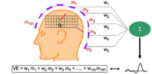
Figure 2 : Beamforming in MEG/EEG. The weights are chosen so as to enhance the neural signal from q0 and suppress or attenuate the signals from elsewhere. Figure modified from [3]
How to choose the weights ?
There are several approaches to choosing the weights, depending on the objective in using the beamformer [1]. In this post, we will focus on a class of beamformers known as linearly constrained minimum variance (LCMV) beamformers, which is widely used in MEG/EEG source estimation. The aim of an LCMV beamformer is to choose the weights such that the output variance (or equivalently the power) of the beamformer is minimized, under the constraint that only the neural signal from the desired location is passed. Thus, what an LCMV beamformer achieves in effect is to preserve the signal from the desired location (q0 in the figure above), while minimizing the contribution to the output from signals that are of no interest (i.e. interfering signals). Mathematically, this is written as
![]()
Where ![]() is the output power of the beamformer and R is the MEG/EEG data covariance matrix. The constraint
is the output power of the beamformer and R is the MEG/EEG data covariance matrix. The constraint ![]() ensures that the neural signal from location q0 is passed to the output with unit gain, where H(q0) is the lead-field matrix for location q0 with three columns, containing EEG/MEG measurement due to unit dipole placed in a three-dimensional source-space in x, y and z direction respectively. Solution to this minimization problem can be found for example using Lagrange multipliers and gives the strength of the neural activity at q0. For more details see [2]. This procedure is repeated for every point/location in the source space (either the cortical surface or the whole brain). By computing the variance or strength or neural activity as a function of location in the source space, source locations can be estimated, with regions of high variance contributing to most of the EEG/MEG measurements , while regions with small variance considered inactive [2].
ensures that the neural signal from location q0 is passed to the output with unit gain, where H(q0) is the lead-field matrix for location q0 with three columns, containing EEG/MEG measurement due to unit dipole placed in a three-dimensional source-space in x, y and z direction respectively. Solution to this minimization problem can be found for example using Lagrange multipliers and gives the strength of the neural activity at q0. For more details see [2]. This procedure is repeated for every point/location in the source space (either the cortical surface or the whole brain). By computing the variance or strength or neural activity as a function of location in the source space, source locations can be estimated, with regions of high variance contributing to most of the EEG/MEG measurements , while regions with small variance considered inactive [2].
In the next blog post we look at some of the assumptions underlying LCMV beamformers and their implications in EEG/MEG inverse problems.
[1] Van Veen, Barry, and K. Buckley. “Beamforming techniques for spatial filtering.” Digital Signal Processing Handbook (1997): 61-1.
[2] Van Veen, Barry D., et al. “Localization of brain electrical activity via linearly constrained minimum variance spatial filtering.” IEEE Transactions on biomedical engineering 44.9 (1997): 867-880.
[3] Hillebrand, Arjan, and Gareth R. Barnes. “Beamformer analysis of MEG data.” International review of neurobiology 68 (2005): 149-171.