Wavelets overcome limitations of methods such as the fourier transform by enabling a view of changes across both time and frequency. Here is a primer on how they can be used for EEG Analysis.
Commonly used techniques such as the Fourier transform assume the signals to be stationary (i.e. consistent in its properties across time) and compute one power spectra for the entire time window. However, it is well known that brain signals are highly dynamic and non-stationary, which means that features such as power spectra can change with time.
Limitations of the Fourier Transform
Recall that in order to take the Fourier transform of a signal, we multiply the signal with an exponential function of the form,
![]()
The result of such an operation is that the signal in the time-domain is transformed into frequency domain, where the information about the phase and amplitude of the signal at every frequency is obtained. In order to obtain the power spectrum, which is commonly used in EEG analysis, Welch method can be used.
see related post Factors that Impact Power Spectral Density Estimation
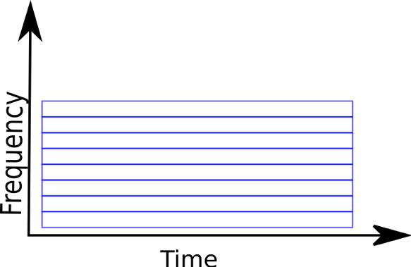
However, we know that EEG signals have very high temporal resolution, on the order of milliseconds and a simple Fourier transform does not exploit this fact. That is, Fourier transform gives information about the amplitude/power of the signal at each frequency, but the information in time is lost (see the illustration below).
From Frequency to Time-Frequency Methods
In contrast Time-frequency (TF) analysis methods such as the short-time Fourier transform and wavelets can be used to reveal the changes in EEG power as a function of both time and frequency.
The basic construct of TF analysis involves dividing an EEG signal into a number of (overlapping) windows. The signal is then transformed into the frequency domain by convolving the signal within the window with a complex function. The result of such a convolution is assigned to the mid-point of the window and the window is moved forward (typically by a sample) and the process repeated. This results in a time-varying power spectrum of the signal. It is important to note however, that this analysis still makes the assumption that the EEG signal is stationary within the window used.
The Short-Time Window Fourier Transform
One straightforward solution to observing changes in the power spectrum over time is to divide the signal up in windows and compute the FT for each window (see illustration below). This method is known as short-time Fourier transform (STFT).
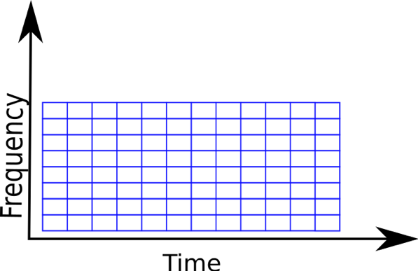
The FT can then be computed for each little window thus giving us the power at each frequency bin, which is averaged for the time interval within that window. One can immediately notice that the STFT gives uniform resolution for all frequencies as it uses windows of fixed size. If the windows are wide, one can get good resolution in frequency but end up with poor resolution in time. Conversely, if windows are narrow, then the signal is better resolved in time, but we lose resolution in frequency. This is a general issue in time-frequency analysis and is known as the uncertainty principle (related to Heisenberg’s uncertainty principle in quantum physics and known as gabor limit in the context of signal processing). Thus, the more precisely you try to localize in time, the more uncertain you get about the frequency and vice-versa.
Wavelets
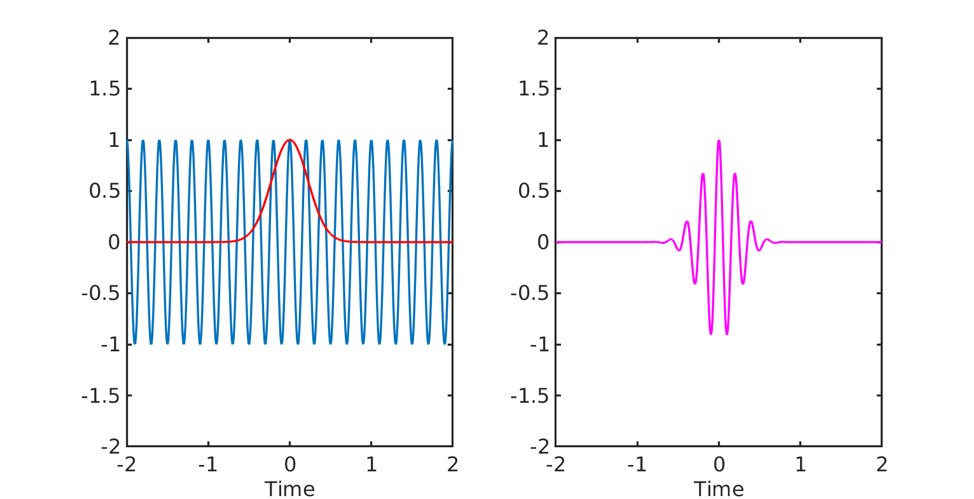
While FT involves equally weighting a signal with a complex sinusoid (actually what we do is convolution! See the equation above) it is possible to design different weighting functions. Using a sinusoid that is active for the entire time window is exactly the problem with FT. Instead what if we could use a signal that is sort of like a sinusoid, but only for a brief period of time and is zero elsewhere? For instance, we could multiply a sinusoid with a gaussian resulting in a signal that is only briefly ‘active’ (see the equation and figure below where f is the frequency of the wavelet and σ the support or spread).
![]()
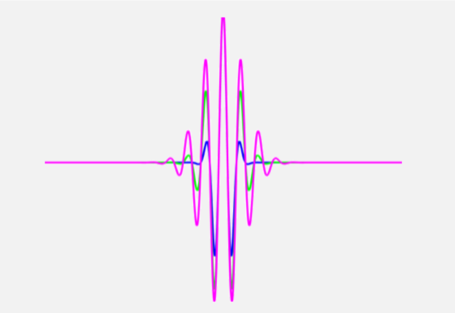
The above function is known as the Morlet wavelet. It is most commonly used in the TF analysis of an EEG signal. The figure below shows the visualization of a Mortlet wavelet obtained by multiplying a sinusoid with a Gaussian.
Note that a wavelet is actually a complex quantity as it is obtained by multiplying a complex sinusoid with a gaussian. The figure above only shows the real parts of the complex quantities for the sake of visualization.
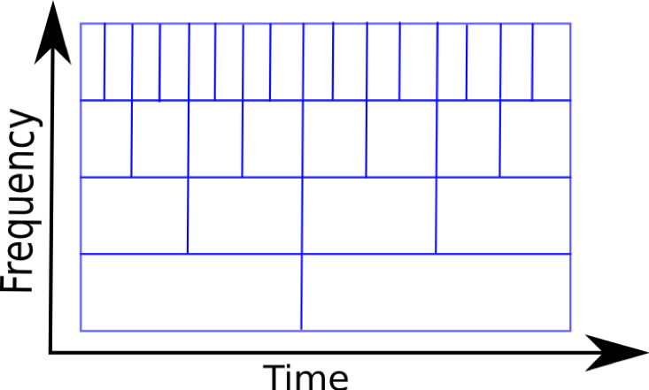
Wavelet transformation then essentially involves convolving the complex wavelet with the EEG signal and moving it along the time axis (known as translation) and doing this with wavelets of varying frequencies (known as scaling; high scale -> low frequency, low scale -> high frequency). Thus higher frequency wavelets can achieve better localization in time, while low frequency wavelets lose some information in time as they are stretched out. Unlike the STFT which has a fixed window size throughout, with wavelets we can analyze a signal at different frequencies with different resolutions. As seen in the figure below, wavelets can provide good frequency resolution and relatively poor temporal resolution at low frequencies, while good temporal resolution and relatively poor frequency resolution at high frequencies.
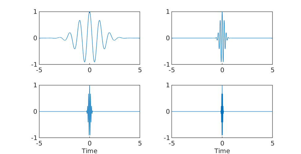
The figure below shows wavelets of frequency 1, 5, 10 and 20 Hz. It can be seen that as the frequency increases the wavelet becomes narrower in time!
Parameters of Morlet Wavelets
The most important parameter that affects the TF decomposition with Morlet wavelets is the number of cycles. Recall that to create a wavelet, we multiply a complex sinusoid with a gaussian and the gaussian function is defined as follows
![]()
Where the spread or width of the Gaussian depends on the number of cycles, via the relation

Now, let us think what happens as we vary the number of cycles for this gaussian. Let’s just plot these gaussians with different cycles in the time and frequency domains.
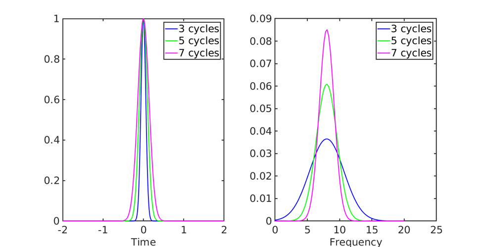
As the number of cycles (n) is increased the width of the Gaussian increases (See Figure above, left). When we take the FFT of these Gaussians (Figure above, right), we see that the Gaussian with lower number of cycles is spread more in the frequency domain compared to the Gaussian with higher number of cycles. For the above examples we set f=8 Hz (i.e., the wavelet frequency) so the Gaussian with n=7 is still more concentrated around 8 Hz compared to lower values of n, but is also more spread out in time!
Choosing the number of cycles
The figure below shows Morlet wavelet with different cycles. Again, the wavelet with higher n has wider spread than wavelet with lower n, which can be interpreted as poorer temporal localization as n increases.
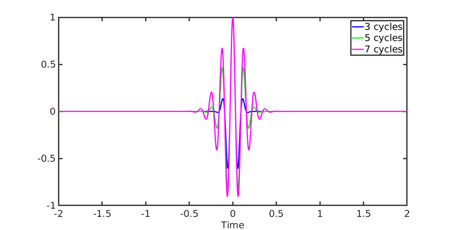
Thus as we get more precise in frequency (with a higher number of cycles), we get more uncertain in time. The figure below shows the corresponding wavelets with number of cycles. So how does one then choose the number of cycles? This really depends on what you are trying to answer with your analysis. If you are more interested in what is happening temporally, for example what happens at 100 ms vs 120 ms, then choose a lower number of cycles. On the other hand, if your interest mainly lies in comparing what happens at 9 Hz vs 15 Hz, then go for a wavelet with higher number of cycles.
Some final caveats
As mentioned before, TF analysis assumes that the EEG signal is stationary within the window, which can be typically in the range of few hundreds of milliseconds. If this assumption is violated then we run into the same problems as with standard FT analysis. Another assumption that TF analysis makes, which is also common to standard FT analysis, is that the brain signals are sinusoidal/rhythmic in nature. While there may be rhythmic components at times, this has been challenged as a general notion [1].
References
- Cole, Scott R., and Bradley Voytek. 2017. “Brain Oscillations and the Importance of Waveform Shape.” Trends in Cognitive Sciences 21 (2): 137–49.