The Alpha Energy metric specifically characterizes the periodic alpha components of the EEG that shows up as a peak above the background decay of the power spectrum. The metric is independent of the shape of the background decay and is sensitive to very small peaks.
Structure of the EEG Signal
The power spectrum of the EEG signal is typically a decreasing function that approximates a 1/f pattern. The shape and slope of this decay can both fluctuate within and between individuals. For example, one study has estimated slopes ranging from 0.5 to 2.25 across individuals and conditions [1]. The basis of this 1/f like structure in EEG has been widely debated. In general however, such structure reflects complex temporal correlations between frequencies and a complex relationship between them that does not lend to a simple interpretation of underlying periodic activity. That said, beyond this most likely non periodic decay, there are periodic/oscillatory components that arise under certain circumstances. The alpha oscillation of course is the most well known, showing up dominantly when one’s eyes are closed, though it can occur under other circumstances as well such as certain eyes open tasks. This periodicity typically shows up as a peak in the power spectrum (though other non-sinusoidal elements can turn up as peaks as well so be careful of your assumptions – see Brad Voytek’s work for examples of that).
see related post The Blue Frog in the EEG
Characterizing the Alpha Oscillation
For the purpose of demonstration let’s take just the alpha oscillation. The traditional way of assessing the alpha oscillation is to simply look at the total alpha band power. However this confounds the background decay and the oscillatory component that contributes to the peak. In some eyes closed situations, the peak is huge compared to the background so the alpha band is a reasonable approximation. However, this is not always the case. Sometimes the oscillation is very weak and shows up as a very small peak. In this case the alpha band will be largely dictated by the background decay. Thus to get a better view of how much of a peak emerges above the background you need to separate the decay from the peak. One way to do this of course is to fit a curve to the background and subtract it from the PSD (see [2] for a good method description of this). This is entirely possible and can do a pretty good job but can perform poorly if the background is a nonuniform kind of function. Also, it is complicated when different subjects have different PSD shapes. Another way to do it is to compute a metric which has been called the Alpha Energy (or more generally oscillation energy if the peak of interest is in another frequency band). This metric is largely independent of the specific shape of the background decay and is much more sensitive to characterizing small peaks.
see related posts Alpha Oscillations and Attention and Alpha, Alpha Everywhere but What Does it Mean?
Computing Alpha Energy
Computing alpha energy has five steps which are also outlined in [3] (or Download the paper here):
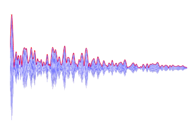
- Compute the PSD: Note that the result you get will depend on the algorithm you use to compute the PSD – the welch method will give you different results from an FFT^2 for example since it averages the windows differently. (See related post Factors that Impact Power Spectral Density Estimation). We prefer to do this as the FFT of the autocorrelation since the autocorrelation itself provides a visualization of periodicity and a sanity check of your result. See panels A-C in the Figure below which provide examples of autocorrelations of different EEG recordings and D-F which are the corresponding PSDs (Figure from [3]).
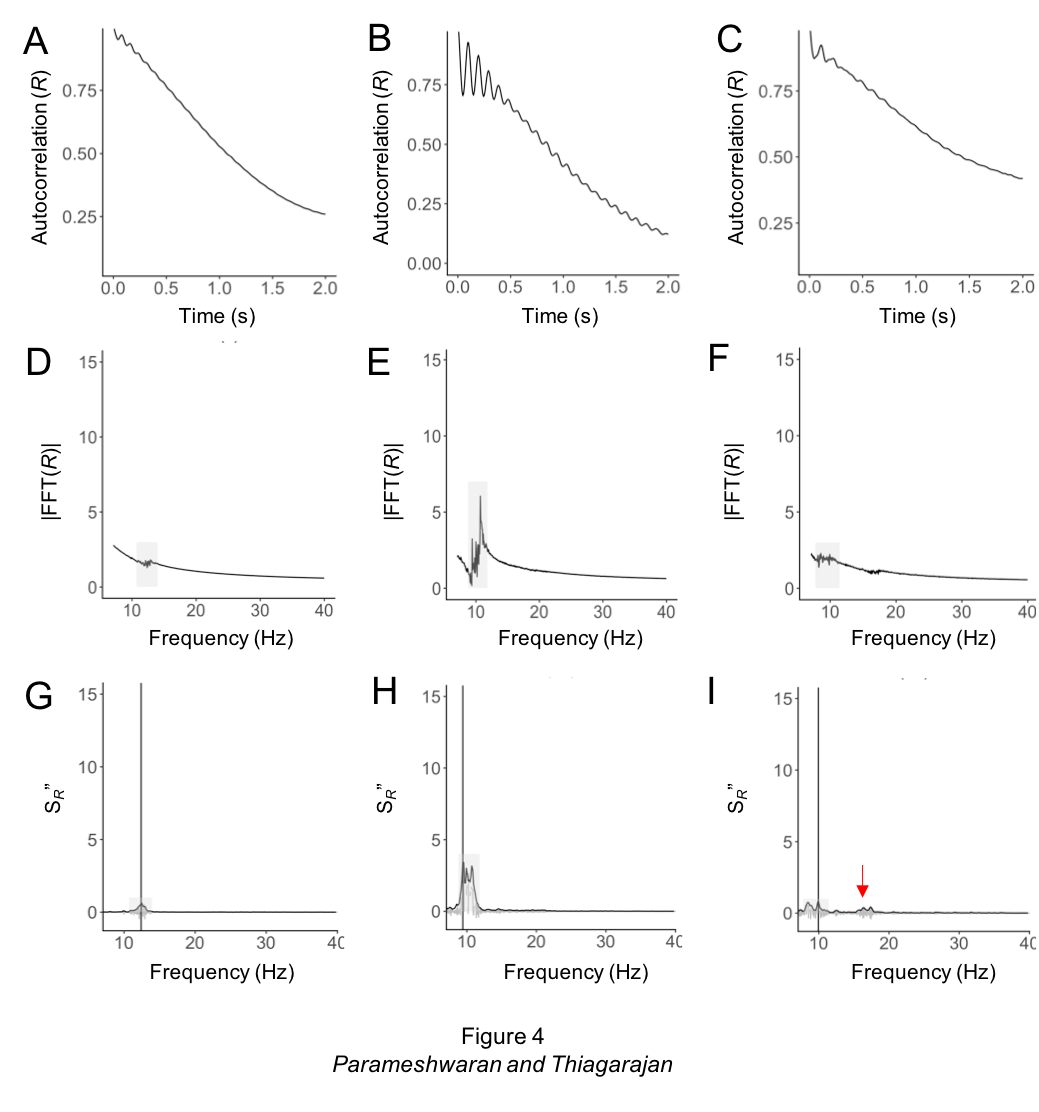
- Compute the second derivative – or actually difference function – of the PSD: This is a method commonly used in spectroscopy to get rid of the slow decay component to look at peaks. It works because the difference in a slow decay is very small while peaks have large differences so what happens is that the decay turns into a roughly straight line and the peak is amplified. The higher order derivative you take the more it will amplify the peak. The second order is good for EEG and will detect most small peaks. The good thing is that it does not matter how the background decay is shaped as long as it is a more gradual decrease/ decay than the peak.
- Compute the Hilbert Envelope of this difference function. The Hilbert envelope serves to create a smooth peak since the difference function will be pretty noisy (i.e. a lot of up and down), a factor that depends to some degree on the parameters of your PSD algorithm. The envelope is the black line in panels G-I (which each correspond to the panels directly above)
- Identify segments of the Hilbert Envelope which are above 1SD of the overall envelope. These segments represent the peaks essentially (shown by grey shading in panels G-I). Sometimes (such as in the case shown in panel C,F,I) you may have multiple peaks and therefore multiple segments. These are shown as the region of the shaded grey bar in G-I above.
- Compute the sum of the Peak Segment (segment of Hilbert envelope >1SD). This is the Alpha Energy or more generally the Oscillation energy and represents essentially the oscillation signal that exceeds the background decay. You can also think of it as a signal to background kind of metric. You can also use this to find the peak frequency which corresponds to the max of a segment minus 2 (minus 2 since we have used the second derivative) represents the peak frequency.
Assumptions
There are a few assumptions to be made in the algorithm:
- The method of computing PSD – this will have the biggest impact on your result
- The smoothing window used to compute the Hilbert envelope – 4 data points seems to be optimal – see [3] for an exploration of this parameter space.
- The SD (standard deviation) threshold of the Hilbert envelope used to choose the segments – 1SD seems to be optimal. Below 0.75 is likely too low and the algorithm will fail because it will pick out too much of the envelope. Above 1SD and up to 2SD is probably fine and won’t make much difference so 1SD is probably a good choice.
Alpha Energy Versus Alpha Band Power
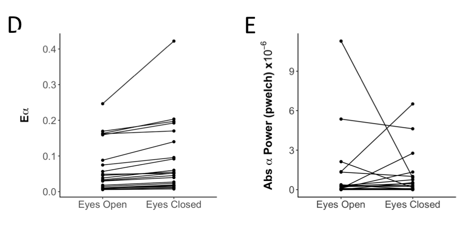
The following example shows how use of the Alpha Energy metric compares to Alpha Band power for a set of people for whom the alpha oscillation was not very strong with eyes closed. While the Alpha Energy (left) was consistently increased for each individual (each individual is a line) the Alpha Band power (right) decreased for some and increased for others due to changes in the background decay.
We have code which we are happy to share. It should be on github soon and we will link it. In the meantime, send us an email.
References
[1] B. Voytek, M.A. Kramer, J. Case, K.Q. Lepage, Z.R. Tempesta, R.T. Knight, and A. Gazzaley,
Age-Related Changes in 1=f Neural Electrophysiological Noise. J Neurosci 35 (2015) 13257{65}.
[2] M.D. Haller, T.; Peterson E.; Varma, P.; Sebastian, P.; Gao, R.; Noto, T; Knight, R.T.; Shestyuk,
A; Voytek, B., Parameterizing neural power spectra. BioRxiv (2018).
figure is from [3]
Thanks for the catch – its fixed now.