EEG analysis often involves estimation of the power spectral density or PSD. Various parameters can impact the results and must be chosen carefully.
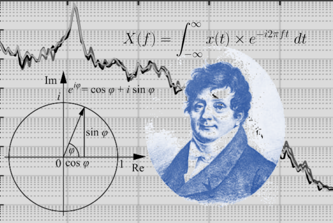
Estimating the power in different frequency ranges is the most ubiquitous analysis performed in the EEG literature. This requires a transformation of the EEG time series from the time domain to the frequency domain. The power spectral density (PSD) is typically estimated using a (discrete) fourier transform or DFT, which provides information about the power of each frequency component. Programming languages like MATLAB, python and R provide ready-made implementation of functions to compute the DFT for a given signal or time series, using the fast Fourier transform (FFT) algorithm. Estimation of PSD depends on various parameters like window length, percentage of overlap between the windows and number of DFT points. It is important to understand how changing these parameters can impact the final result.
Sample data:
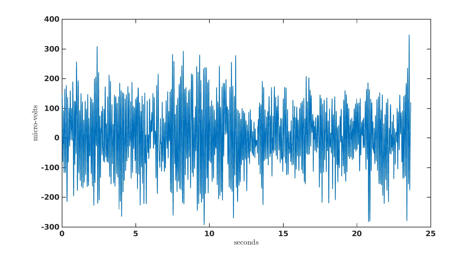
To illustrate the effect of the above mentioned parameters on PSD estimation, we will use data from this website as an example. The data contains EEG recordings from a subject with eyes closed and has 4097 sampless sampled at 173.15 Hz. The figure below shows data from a single channel.
Estimating PSD with FFT
Power spectral density (PSD) can be estimated by computing the magnitude squared of its DFT. In MATLAB, this is achieved by simply using the command fft() (see the code below). The fft() command basically needs two inputs – the signal vector (x) and number of DFT points (N). The parameter N determines the frequency resolution (how many Hz each DFT bin represnts) of the spectrum based on the sampling frequency which is given by freq_res = (f_s / N).
Choice of N in fft()
Due to the way the FFT algorithm works, the convention is to set N to the power of 2 that is next above the length(x). For instance, if length(x) is 1000, then N = 1024 (2^10). Although, this is not mandatory, it just makes for an efficient and faster implementation of FFT. However, it is recommend not to set N < length(x), because FFT will then utilize only the first N samples of the data to estimate the PSD and truncate rest of the data.
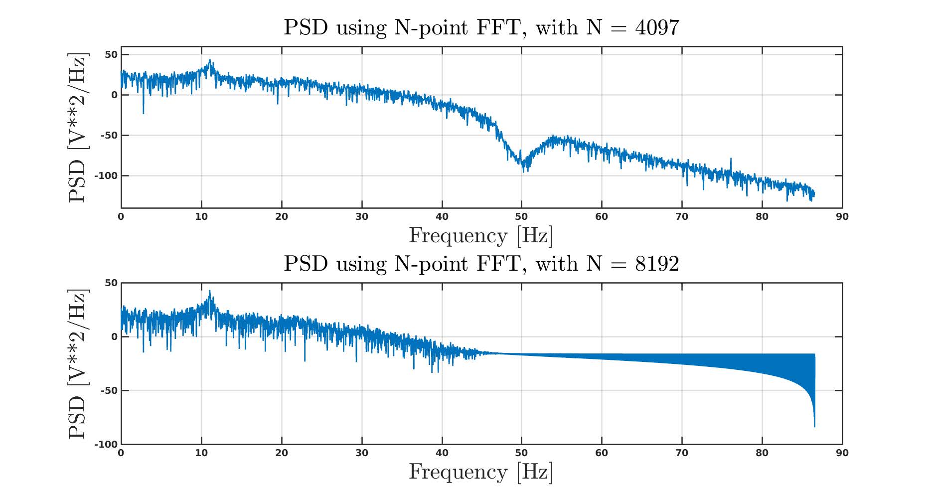
It is pretty evident from the figure above that the PSD estimate obtained using FFT is quite noisy and jagged, with many different frequencies contributing to the signal. Also what is known as 1/f behavior is apparent from the above plot, where lower frequencies contribute to most of the power in the signal and higher frequencies have low power content.
Estimating PSD with the Welch method
The Welch method is another commonly used to estimate PSD from EEG. The basic idea behind the Welch method is to use a moving window technique where the FFT is computed in each window and the PSD is then computed as an average of FFTs over all windows. This is achieved by using the pwelch() command in MATLAB.
Estimation of PSD by Welch’s method depends on three parameters, 1) window length – win, 2) percentage of window overlap – noverlap and 3) number of FFT points – N. In addition to this, one can also choose different windowing functions, but the Hanning window is most widely used as it has good frequency resolution and reduced spectral leakage. So for the purpose of this post, we will stick to Hanning window!
We have already described the role of N. Thus, for the remainder of the post, we will simply assume that N is set equal to the length of the window. Now let us understand how the choice of these two parameters – 1) win and 2) noverlap affect your PSD estimates.
Effect of varying the window size
The number of segments the entire data will be divided into is determined by win and noverlap. First let us set the noverlap to 50% (Note that in MATLAB noverlap is typically specified in samples. So 50% overlap translates to 0.5*win) to illustrate the effect of varying window sizes. Let’s choose win to be 0.25 seconds, 1 second and 5 seconds. For the given example data this roughly translates into window sizes of 45, 174 and 880 points respectively.
It is obvious that a smaller window size will increase the total number of windows the data will be divided into. This will help in obtaining smooth PSD estimates because the random effects of noise is averaged out. However, the downside to a smaller window size (which is used to set the value of N) is that the frequency resolution is compromised as the distance between two frequency points increased and this results in lower frequency resolution (recall that freq_res = (f_s / N) ).
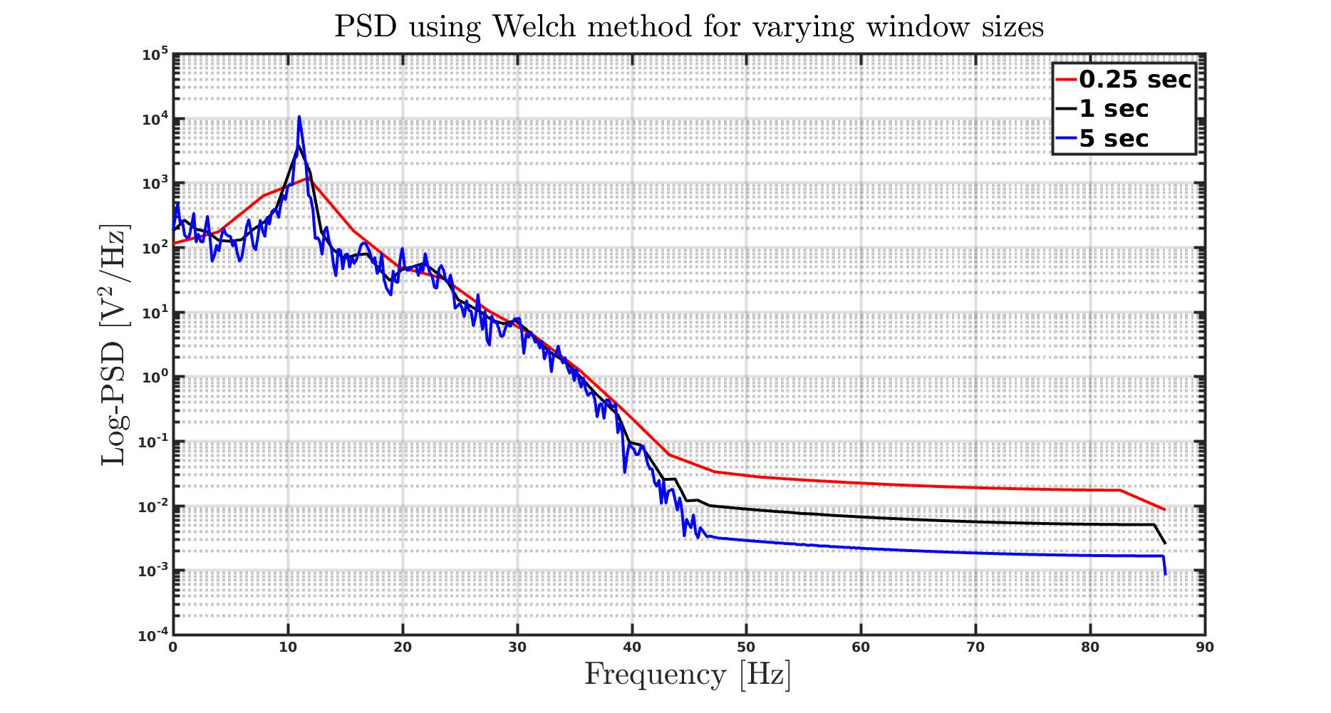
This fundamental point is evident from the figure below where we can see that when the window size is approximately 0.25 seconds (approximately 45 samples), we obtain a very smooth PSD (due to higher number of windows to average
from), but with low frequency resolution (as indicated by the wide peak between 5 and 15 Hz that represents the common eyes closed Alpha Oscillation which you can read about here) .
Conversely, by increasing the win to 1 second (approximately 174 samples), we have improved the frequency resolution and thus we can see that we get a narrower lobe (ranging between 8 and 13 Hz), centered around 11 Hz. Although the total number of
windows has now decreased due to increased window length, it is still large enough to cancel the effects of random noise. On further increasing the window size to 5 seconds (approximately 880 samples), we note that the PSD estimates have only slightly sharper frequency resolution but get noisier as effects of noise is not canceled out due to smaller number of windows!
Effect of varying the overlap percentage
To illustrate the effect of varying noverlap (0%, 25%, 50% and 75%), let us set win to 3 seconds (which translated to approximately 500 samples, which is also the number of DFT points in our case). The results are shown below. Note that with 0% overlap, the PSD is relatively more noisy and bumpy compared to for example 50 % overlap. By increasing the overlap percentage (for a given window size), we increase the total number of windows, which helps in averaging out the effects of noise. However, there is a limit to this.
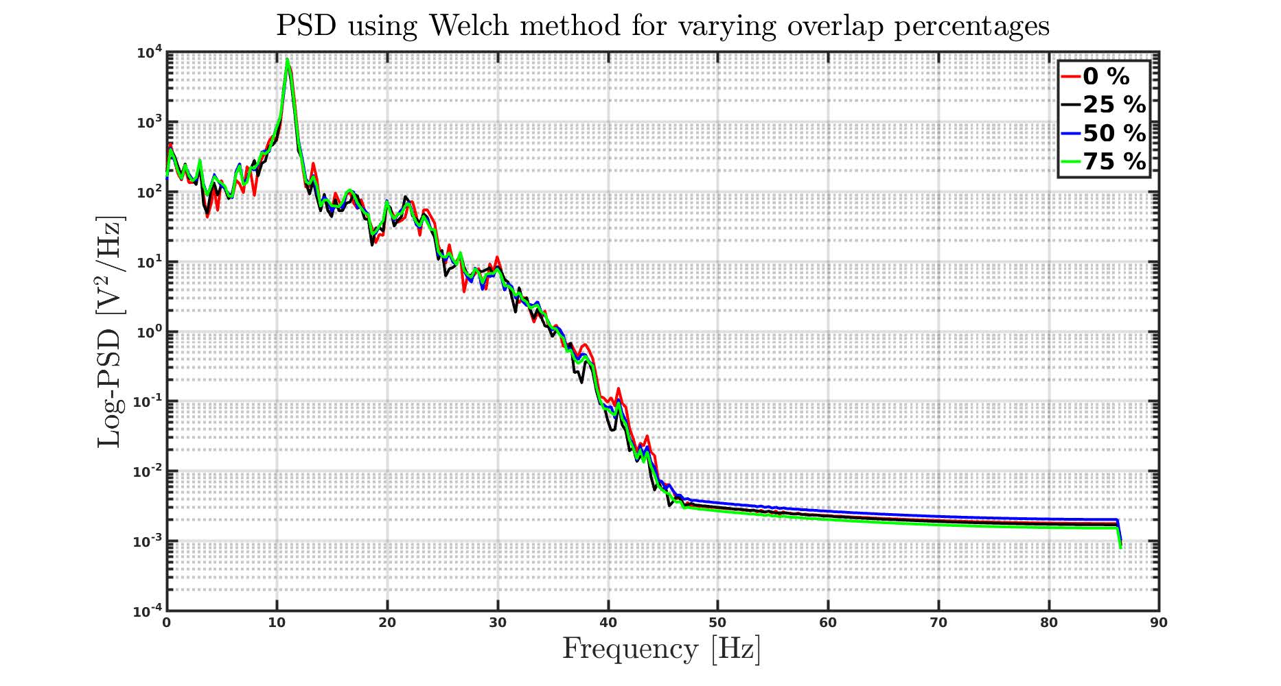
Increasing the overlapping percentage to 90% or even 99% may not help much due to high correlation between the window samples and thus averaging will not cancel the effect of noise. In the case of our example data, we can see that there is not much of a difference between 50% and 75% overlap.
Summary
The Fourier transform is a fundamental tool for EEG signal analysis. But care must be taken in choosing the right parameters depending on the nature of your EEG data. Following key points must be kept in mind
1) By using Welch method one can obtain smoother PSD
2) Choosing very short windows to compute PSD can lead to poor results, particularly if you have short epochs and you are interested in analyzing lower frequencies.
3) Longer windows can result in finer resolution of PSD, but can lead to noisy PSD. One needs to strike a balance here, depending on the frequencies of interest.
4) The number of DFT points should always be greater than or equal to the length of your data or window.
5) Highly overlapping windows does not guarantee smoother PSD estimates due to high correlation between the windows.
See related post The Blue Frog in the EEG
Try it yourself with this MATLAB code:
PSD with FFT
%psd with FFT using N = length(x) and nextpow2(length(x))
% xout – EEG data from single channel
figure
set(groot,’defaulttextinterpreter’,’latex’);
m = [length(xout), 2^(nextpow2(length(xout)))];
for i=1:1:length(m);
N = m(i);
xdft = fft(xout,N);
xdft = xdft(1:N/2+1);
psdx = (1/(fs*N)) * abs(xdft).^2;
psdx(2:end-1) = 2*psdx(2:end-1);
freq = 0:fs/N:fs/2;
subplot(2,1,i)
plot(freq,10*log10(psdx))
text_t = sprintf(‘PSD using N-point FFT, with N = %d’, m(i));
title(text_t, ‘FontSize’, 24)
xlabel(‘Frequency [Hz]’, ‘FontSize’, 24′)
ylabel(‘PSD [V$^2$/Hz]’, ‘FontSize’, 24)
grid on
end
PSD with Welch
%psd for varying windows
set(groot,’defaulttextinterpreter’,’latex’);
win=[ceil(0.25*fs) ceil(1*fs) ceil(5*fs)];
col = {‘r’, ‘k’, ‘b’};
for i=1:1:size(win,2)
nfft = win(i);
noverlap = 0.5*win(i);
[pxx,f] = pwelch(xout,win(i),noverlap,nfft,fs,’onesided’);
length(f)
%figure
semilogy(f, pxx, col{i})
hold on
grid on
legend(‘0.25 sec’, ‘1 sec’, ‘5 sec’, ‘FontSize’, 24)
end
xlabel(‘Frequency [Hz]’, ‘FontSize’, 24)
ylabel(‘Log-PSD [V$^2$/Hz]’, ‘FontSize’, 24)
title(‘PSD using Welch method for varying window sizes’, ‘FontSize’, 24)
%psd for varying overlap percentages
win = ceil(3*fs);
nfft = win;
noverlap_pc=[0 0.25 0.5 0.75];
noverlap = ceil(win*noverlap_pc);
col = {‘r’, ‘k’, ‘b’, ‘g’};
figure
for i=1:1:size(noverlap_pc,2)
[pxx,f] = pwelch(xout,win,noverlap(i),nfft,fs,’onesided’);
length(f)
%figure
semilogy(f, pxx, col{i})
hold on
grid on
legend(strcat(num2str(noverlap_pc(1)*100),’ %’), …
strcat(num2str(noverlap_pc(2)*100),’ %’), …
strcat(num2str(noverlap_pc(3)*100),’ %’), …
strcat(num2str(noverlap_pc(4)*100),’ %’),’FontSize’, 24)
end
xlabel(‘Frequency [Hz]’, ‘FontSize’, 24)
ylabel(‘Log-PSD [V$^2$/Hz]’, ‘FontSize’, 24)
title(‘PSD using Welch method for varying overlap percentages’, ‘FontSize’, 24)

How can I cite this page?
Title and authors name with a link should work – maybe as follows:
Factors that Impact Power Spectral Density Estimation, Narayan P. Subramaniyam, Lab Talk, Sapien Labs + url
Good work! Thank you for providing such a clean code!
Thank you for providing such a comprehensive overview!
You helped me understand PSD better.
I have one question: In your example code with varying window size, the Y-axis of the figure is labeled ‘Log-PSD’.
I’m having a hard time understanding where the logarithm comes into play, as it is not in the example code. Is this something the pwelch function does automatically (I also cannot seem to find it in that documentation)?
(Sorry for obvious questions, I have no engineering background, but trying to grasp what PSD exactly does)
Thank you!
Hi. Thanks for your comment. It comes from here : semilogy(f, pxx, col{i}).
I am using semilogy function in matlab, that makes y-axis log-scale.
Please if I want to reference, which year is should I use. thank you
Regarding the choice of N, if I have a dataset of say 10K, then would the nfft value be set to 16384 (2^13)? The example clearly illustrates the tradeoff between spectral resolution and noise reduction with the window size. Are there any conventions or common practices for selecting window sizes with welch’s methods of psd estimation?
Hi, in practice NFFT must be greater than your series length but fft algorithm is more efficient when it is the power of 2 which is greater or equal to the number of samples of the signal. So in your case with 10000 points it is enough if NFFT = 16384 (i.e., 2^14). Remember that when NFFT > L the signal is zero padded to the NFFT length, but because of the nature of fft algorithm it is fastest for powers of two.
More info : https://se.mathworks.com/help/matlab/ref/fft.html