EEG microstates represent a dynamical view of how the spatial distribution of the electric potential on the scalp changes over time. Microstates typically last 80-100 ms.
Traditional analysis of EEG signals involves frequency domain analysis using fast Fourier transform or time-frequency analysis using wavelets. An alternative way of analyzing EEG is to take the dynamical systems approach such as (for example lyapunov exponents), and view it in terms of state and dynamics. State variables are the minimum number of variables required to fully describe a dynamical system (for example, a pendulum can be fully described by its angular position and velocity) at any given time t, and the dynamics describes how the state changes or evolves over time. Microstate analysis of EEG, introduced in Lehman et al. [1] falls in the category of dynamical systems analysis. It defines the states as the topographies of electric potential over all the EEG electrodes, essentially a view of the spatial distribution of the electric potential on the scalp at each time point. It is assumed that different distributions of neuronal generators in the brain give rise to different configurations of potential maps on the scalp [2]. Thus studying the changes in the configuration of the topography (i.e. state variables) over time (i.e. dynamics), reflects the changes in the activity of large-scale neuronal networks and this is the rationale behind microstate analysis.
Microstate analysis of resting-state EEG
Multichannel EEG measures the activity of large-scale neuronal networks with millisecond resolution. Several studies have shown that large-scale networks are not just involved in attentive tasks, but also during spontaneous cognitive activities that are stimulus-independent [3], for example such as resting-state EEG.
Lehman et al. [1] showed that the alpha frequency band of the resting-state EEG is composed of a discrete number of, what is defined as ‘quasi-stable’ states and gave them the name microstates. Essentially, each microstate is a topography of electric potential over EEG electrodes, which remain stable for a certain duration, before jumping or transitioning into a new and distinct topography. Thus the topographical maps configuration do not evolve in time randomly and continuously, but in a rather discrete and abrupt fashion, after remaining stable for a certain duration. Also, within the period of this stable time window, the strength of the field increases and decreases, but the topography remains the same.
In order to obtain EEG microstates from resting-state or spontaneous EEG, global field power (GFP) is computed, which can be considered as a reference-independent, single measure of response strength to an event or any change in the brain activity [4] and it is simply given as the root mean square across average-referenced electrode values at a given time instant,
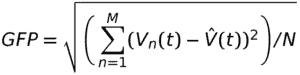
where Vn (t)is the electric potential at electrode i at time t and V^(t)is the average over M electrodes at time t. Another way of interpreting GFP is as the spatial standard deviation of the signal. Interestingly, the topographic maps tend to be most stable around the (local) maxima of the GFP (i.e. where the spatial variability across channels is highest). Such topographies at the local maxima of GFP are considered as discrete states in EEG microstate analysis, an example of which is shown in the Figure below from Khanna et al. [5] for resting-state (eyes closed) EEG data. GFP is plotted as a function of time.
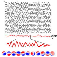
Figure 2 : Resting-state EEG along with the GFP shown in red. Topographies at local maxima of a certain section of GFP is also shown in the last row (from [5]) .
Note that microstate analysis can be impacted by the choice of reference, as the instants of the GFP peaks due to different references will influence the microstates topographies. Although, average reference is commonly used, a recent study based on simulations and real EEG data, have shown that REST reference may show better performance compared to average reference in identifying microstates features [10].
A few topographies dominate
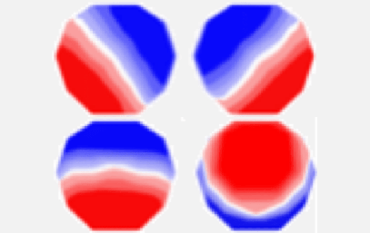
Several studies have shown that, although a large number of topographic maps can be obtained from EEG recordings, about 70-80% of the variance in these maps is explained by just a few topographies. Surprisingly, several studies have shown that shown that, usually around four topographies account for most of the variance (>70%) in these maps [7] . These four microstate class topographies are shown in the figure below. These are right-frontal left-posterior (A), left-frontal right-posterior (B), midline frontal-occipital (C), and midline frontal topographies (D). Also, the microstates typically last between 80-120 ms before jumping into another state. Other studies have also found microstates beyond these four prototypical maps, but it has been shown that at most 8 classes of distinct topographies dominate resting-state EEG [8-9].

Figure 3 : Four prototypical microstate classes that account for most of the variance in resting-state EEG (from [5]).
In a study by Koenig et al. [6] et al., microstate analysis of resting-state (spontaneous) EEG from 496 subjects in different age range (6-80 years) revealed that four dominant microstates had mean duration around 80-100 ms, with children (6-12 years) having comparatively longer duration, which tends to stabilize around adulthood [5].
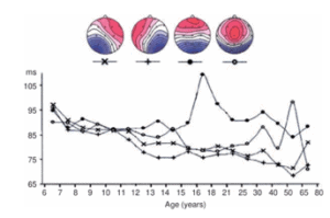
Figure 4 : Mean microstate duration for 4 prototypical maps [3,6].
How do you define microstates from the GFP maxima?
Given a wide array of topographic maps, how do we find a group of maps that account for the most variance in the data? One way to obtain a solution to this problem is to use clustering approach and several clustering algorithms such as K-means, principal component analysis, hierarchical clustering or agglomerative clustering, Gaussian mixture models, to mention a few can be used. There are several considerations to these clustering approaches such as threshold decisions which can impact results. These aspects which will be addressed in a subsequent post with a more detailed view of extracting microstates.
References
[1] Lehmann, D.; Ozaki, H.; Pal, I. (1987). “EEG alpha map series: Brain micro-states by space-oriented adaptive segmentation”. Electroencephalography and Clinical Neurophysiology. 67 (3):
[2] Michel, C. M., & Koenig, T. (2018). EEG microstates as a tool for studying the temporal dynamics of whole-brain neuronal networks: a review. Neuroimage, 180, 577-593.
[3] Michel, C. M., Koenig, T., Brandeis, D., Wackermann, J., & Gianotti, L. R. (Eds.). (2009). Electrical neuroimaging. Cambridge University Press.
[4] Skrandies, W. (1990). Global field power and topographic similarity. Brain topography, 3(1), 137-141.
[5] Khanna, A., Pascual-Leone, A., Michel, C. M., & Farzan, F. (2015). Microstates in resting-state EEG: current status and future directions. Neuroscience & Biobehavioral Reviews, 49, 105-113.
[6] Koenig, T., Prichep, L., Lehmann, D., Sosa, P. V., Braeker, E., Kleinlogel, H., … & John, E. R. (2002). Millisecond by millisecond, year by year: normative EEG microstates and developmental stages. Neuroimage, 16(1), 41-48.
[7] Lehmann D, Pascual-Marqui RD, Michel C. EEG Microstates. Scholarpedia. 2009; 4:7632
[8] Wackerman J, Lehmann D, Michel CM,Strik WK. Adaptive segmentation of spontaneous EEG map series into spatially defined microstates. International Journal of Psychophysiology 1993;14:269–283.
[9] Strik, W. K., & Lehmann, D. (1993). Data-determined window size and space-oriented segmentation of spontaneous EEG map series. Electroencephalography and Clinical Neurophysiology, 87(4), 169-174.
[10] Shiang Hu, Esin Karahan, Pedro A. Valdes-Sosa Restate the reference for EEG microstate analysis https://arxiv.org/abs/1802.02701