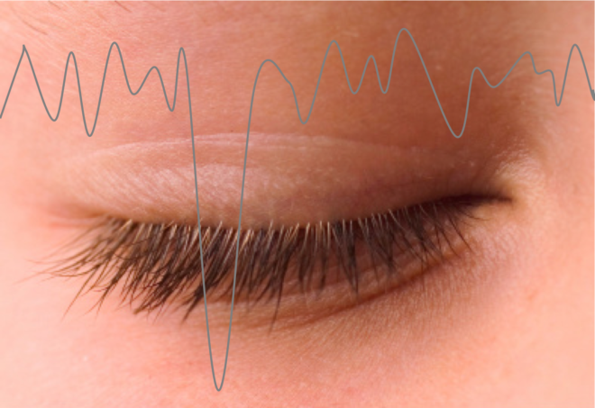
The eye blink is one of the most common contaminants of the EEG signal. Here we discuss some common techniques used to remove it including linear regression and Independent Component Analysis.
One of the challenges of EEG is that the surface electrodes also pick up the electrical activity of muscle contraction on the face (the electromyograph or EMG). While a subject can be asked to try and not change their facial expression too much, the eye blink or Electro-oculographic (EOG) simply can only be controlled so much. It is therefore one of the biggest contaminating signals and can greatly hinder the interpretation of EEG signals. The eye blink is characterized by a sharp deflection that is usually strongest at the front of the brain and is easy to recognize. For this reason, many ‘BCI’ or brain-computer interface applications actually make use of the eye blink rather than brain activity. However, if you want to make sure you are studying brain activity alone it is necessary to get rid of it and researchers have come up with many methods to do so. The two most commonly used and popular methods are linear regression and independent component analysis (ICA) which we describe here. Yet despite how easy it may seem to visually ‘see’ the EOG in the signal, specifically removing it has its challenges.
Linear regression
Linear regression algorithms have been commonly used to remove ocular artifacts from EEG data due to their simplicity. This approach typically requires an additional set of electrodes on the face to record electrical activity due to eye blinks and movements.
The main assumption in this approach is that each EEG channel can be expressed as the sum of noise-free EEG signal and a fraction of the source artifact available through EOG electrodes. The aim of the regression approach is then to correct the EOG artifacts by subtracting weighted portion of each EOG channel from the contaminated EEG signal.
Let S be the recorded EEG signal which can be expressed as the sum of noise-free EEG signal E and EOG or eye blink signal B multiplied by a weight matrix W.
S = WB + E
The weight matrix W contains what is known as the regression co-efficients that describes the contribution of the EOG artifact in each EEG channel and has to be figured out and calculated somehow. Once W is known, the noise-free EEG activity is easily obtained by simply subtracting the weighted eye blink B from the signal.
E = S – WB
The most commonly used to method to perform linear regression is the ordinary least squares (OLS) method – essentially imagine fitting a regression line using the mean squared sum of residuals through a scatter of the recorded signal on each channel vs the recorded EOG and finding its regression coefficient. This amounts to estimation of W by minimizing the residuals over all the channels, i.e. minimizing the term (S – WB)T (S – WB) by setting its gradient with respect to W to zero.
One of the major problems with this approach is the assumption that the EOG electrodes do not record any EEG activity, which is simply not true. Since EOG signals which are recorded near the forehead will also record some EEG activity, the OLS method will tend to overestimate W leading to the removal of some EEG activity as well along with the EOG activity.
Independent component analysis
Independent component analysis (ICA) is a blind source separation (BSS) technique that is widely used in an array of signal processing applications. ICA has become quite popular in denoising biomedical signals and is the most preferred / popular method to clean EEG data. It is available in EEGLAB [1] for example, which also provides a nice visualization for ICA analysis.
The intuition behind ICA is best explained using cocktail party problem
 Figure adapted from [5]
Imagine you are at a party where the music is being played and at the same time there is some speech going on (pretty bad party arrangement!). These two sources of sound, let’s call them s1 and s2 are being picked up by microphones m1 and m2. ICA assumes that the sounds s1 and s2 add up or mix linearly and the output of each microphone can be expressed as
m1 = s1 * a1 + s2 * b1
m2 = s1 * a2 + s2 * b2
where a1, b1, a2, b2 are the linear weights describing the contribution of each original sound to the microphone. The goal of ICA is to retrieve the weights and the original sounds s1 and s2. So if one is just interested in listening to the music and wants to get rid of the speech signal, then one simply has to set the weights b1 and b2 to zero in the above equation!
Similarly, in the context of EEG recording, one can thing of EEG electrodes as microphones that are picking up sound from various sources like neural activity, eye activity, muscle activity etc. ICA can thus be used to disentangle these sources, which are called as independent components. Let S be the contaminated EEG signal. ICA assumes the following linear model
S = M*X
Where M is the mixing matrix, that contains the linear weights describing the contribution of neural and various non-neural sources to the EEG recording and X the underlying sources, also known as independent components. ICA seeks to estimate
Xest = W*S
where W is the un-mixing matrix. There are many algorithms to solve the ICA problem (and are readily available in EEGLAB) and the majority of them use higher-order statistics. We will not go into the math or the details of it, but it is important to know that this is an under-constrained problem, meaning that we observe only S and try to estimate M and X so the number of unknowns are more than the observations. It is hence a challenging problem.
It is important to note that ICA methods makes four main assumptions – 1) Summation of sources at scalp electrodes are linear, 2) Artifacts and neural sources are spatially fixed across time, 3) Component activations are temporally independent and 4) Underlying sources are non-Gaussian. In addition, it is also assumed that the number of independent sources are at most equal to the number of recording channels.
The amount of data given to the algorithm plays an important role in ICA. As ICA is based on statistical features, results will not be reliable if the data length is short or insufficient. Romero, Mañanas and Barbanoj have suggested that the length of the data should be some constant times the square of the number of channels [8]. Jung, Makeig and others have shown that epochs of 10s are enough to obtain reliable results [9]. Also, assumption no. 2 may not always be true in practice (neural activity need not be spatially stationary through time) and hence the choice of data length should be such that assumption no. 2 is reasonably satisfied.
Identification of blinks and eye movement components
Once the components have been identified, to remove the EOG artifacts, one can visually determine which independent component corresponds to eye-blinks or movements based on the following criteria.
To identify blink and horizontal eye-movement related components the following properties are typically used,
- Presence of frontal topography (for blinks, shown on left) and bilateral with opposite sign frontal topography (for horizontal eye-movements, shown in right) in scalp map (adapted from here).

2. Flat power spectra with no peaks at physiologically relevant frequencies
 Figure adapted from [2]
- High correlation with vertical EOG recordings (for blinks) or with horizontal EOG recordings in case of horizontal eye-movements.
- Presence of high amplitude in the component.
After identifying the components related to EOG artifacts, the corresponding column in the mixing matrix to M is set to zero, which essentially means zeroing the weights of EOG-related sources to all the EEG electrodes. The noise free EEG can now be obtained as
S = M*Xest

In the figure above (taken from here) one can see that the independent components 1 and 2 are clearly related to EOG artifacts, which is also evident from the scalp maps showing high activity in the frontal sites. Setting these components to zero gets rid of artifacts related to eye-movements as seen in the figure above.
Another point to note is that, as with regression, the components related to EOG activity may also contain some EEG activity and thus in practice there is no guarantee that discarding the EOG related components may not result is throwing away some useful EEG information as well!
Automated selection of components
Since visual identification of artifacts can be very subjective, researches have come up with objective statistical measures to automatically identify EOG-related components. These statistical measures include correlation with EOG electrodes, temporal kurtosis, spatial average and variance difference, maximum epoch variance are available and are implemented in tools like SASICA [2], FASTER [3] and ADJUST [4] which are available as plugins in EEGLAB.
Other methods
Adaptive and Weiner filtering can be used to reduce EOG artifacts. Adaptive filtering is an improvement over simple linear regression where the weights can vary with time unlike in linear regression. Weiner filtering is another filtering approach that aims minimize the mean square error between the desired signal and its estimate using power spectral densities. This approach does not require a reference EOG waveform.
Improvements / extensions to ICA approach have also been suggested. By imposing spatial constraints on the mixing matrix, i.e., prior assumption of the spatial topography of source sensor projections, it has been shown that the performance of ICA in denoising EEG signals can be greatly improved.
Then there are methods such as principal component analysis, signal space projection, cannonical correlation analysis that can be employed for EOG artifact reduction, but ICA is mostly preferred in the EEG community due to its ability to deal with many kinds of artifacts (EOG, muscle artifact, cardiac artifacts, line noise) at once. Although, ICA is widely used, it is important to keep in mind that this approach is also not devoid of pitfalls and makes several assumptions that in practice may not be true. Thus, being aware of these assumptions while choosing the data length and properly classifying artifactual components is critical.
Thus while none of the methods can do a perfect job in removing the eye blink and some EEG signal may be lost in the process, its presence can substantially distort metrics of the signal – particularly metrics like the Hurst exponent or DFA. Thus it is always prudent to do the best job possible.
References
- https://sccn.ucsd.edu/eeglab/index.php
- Chaumon, Maximilien, Dorothy VM Bishop, and Niko A. Busch. “A practical guide to the selection of independent components of the electroencephalogram for artifact correction.” Journal of neuroscience methods250 (2015): 47-63.
- Nolan H, Whelan R, Reilly RB. FASTER: fully automated statistical thresholding for EEG artifact rejection. J Neurosci Methods 2010;192(1):152–62
- Mognon A, Jovicich J, Bruzzone L, Buiatti M. ADJUST: an automatic EEG artifact detector based on the joint use of spatial and temporal features. Psychophysiology 2011;48(2):229–40.
- Shlens, Jonathon. “A tutorial on independent component analysis.” arXiv preprint arXiv:1404.2986(2014).
- Makeig S, Bell AJ, Jung T-P, Sejnowski T. Independent component analysis of electroencephalographic data. Advances in neural information processing systems, vol. 8. Cambridge, MA: MIT Press; 1996. p. 145–51
- Croft R J and Barry R J 2000 Removal of ocular artifacts from the EEG: a review J. Clin. Neurophys 30 5–19
- Romero S, Mañanas M A and Barbanoj M J 2008 A comparative study of automatic techniques for ocular artifact reduction in spontaneous EEG signals based on clinical target variables: a simulation case Comput. Biol. Med. 38 348–60
- Jung T P, Makeig S, Humphries C, Lee T W, McKeown M J, Iragui V and Sejnowski T J 2000 Removing electroencephalographic artifacts by blind source separation Psychophysiology 37 163–78


I don’t see Berg and Scherg Dipole method which is the best. Superior to all methods, Article in Electroencephalography and Clinical Neurophysiology 79(1):36-44 · August 1991
Is there a reference for your (‘best’) claim?
See Article in Electroencephalography and Clinical Neurophysiology 79(1):36-44 · August 1991 with 106 Reads
DOI: 10.1016/0013-4694(91)90154-V
Best and most sensible method